Short Numpy Tutorial

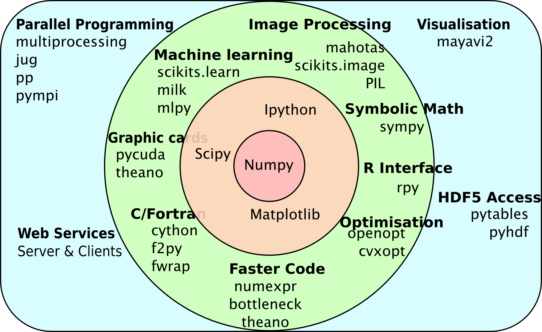
This is a very short introduction to numpy, focused on the basic data structure, ndarray. Numpy is the most important scientific package in the Python ecosystem because it provides a common datastructure on which many other packages build on.

To make this tutorial work on Python 2 & Python 3, let's import some future features into Python 2

from __future__ import print_function, division

# np is the standard abbreviation for numpy in the code
# Even the numpy docs use it
import numpy as np

What is an ndarray?

The ndarray is the biggest contribution of numpy. An ndarray is

• a regular grid of N-dimensions,
• homogeneous by default (all the elements have the same type),
• contiguous block of memory with types corresponding to machine types (8-bit ints, 32 bit floats, 64-bit longs, ...).

Building an array (inline)

We can build an array from Python lists:

arr = np.array([
    [1.2, 2.3, 4.0],
    [1.2, 3.4, 5.2],
    [0.0, 1.0, 1.3],
    [0.0, 1.0, 2e-1]])
print(arr)

Inspecting array properties

print(arr.dtype)
print(arr.ndim)
print(arr.shape)

This array is of float64 (at least on my computer, probably on yours too), it has 2 dimensions and its shape is 4 rows and 3 columns.

When constructing an array, we can explicitly specify the type:

iarr = np.array([1,2,3], np.uint8)

Arithmetic operations on the array respect the type and can including rounding and overflow!

arr *= 2.5
iarr *= 2.5
print(arr)
print(iarr)

Boolean operations

An important subset of operations with numpy arrays concerns using logical operators to build boolean arrays. For example:

is_greater_one = (arr >= 1.)
print(is_greater_one)

Slicing & Dicing

We can use Python's [] operator to slice and dice the array:

print(arr[0,0]) # First row, first column
print(arr[1]) # The whole second row
print(arr[:,2]) # The third column

Slices are views

Slices share memory with the original array!

print("Before: {}".format(arr[1,0]))
view = arr[1]
view[0] += 100
print("After: {}".format(arr[1,0]))

Visual illustration of slicing

a = np.array([
       [ 0,  1,  2,  3,  4,  5],
       [10, 11, 12, 13, 14, 15],
       [20, 21, 22, 23, 24, 25],
       [30, 31, 32, 33, 34, 35],
       [40, 41, 42, 43, 44, 45],
       [50, 51, 52, 53, 54, 55]])

This image is taken from scipy-lectures, a more complete tutorial on numpy than what we have here.

Basic functions on arrays

arr.mean()

Also available: max, min, sum, ptp (point-to-point, i.e., difference between maximum and minimum values).

These functions can also work axis-wise:

arr.mean(axis=0)

An important trick is to combine logical operations with A

is_greater_one = (arr > 1)
print(is_greater_one.mean())

Broadcasting

You can often perform operations

print(arr)
print("Now adding [1,1,0] to *every row*")
print()
arr += np.array([1,1,0])
print(arr)

The exact rules of how broadcasting work are a bit complex to explain, but it generally works as expected. For example, if your data is a set of measurements for a sample, and your columns are the different types of measurements, then, you can easily remove the mean like this:

print(arr.mean(0))
arr -= arr.mean(0)
print(arr.mean(0))

Footnotes

[homogeneous]: There is a loophole to get heterogeneous arrays, namely an array of object. Then, you can store any Python object. This comes at the cost of decreased computational efficiency (both in terms of processing time and memory usage).